Getting Started

Installation guide

To install nnodely, the user can install via:

pip install nnodely

Alternatively, the user can clone the repository and install from source:

git clone https://github.com/tonegas/nnodely.git
cd nnodely
pip install -r requirements.txt
pip install .

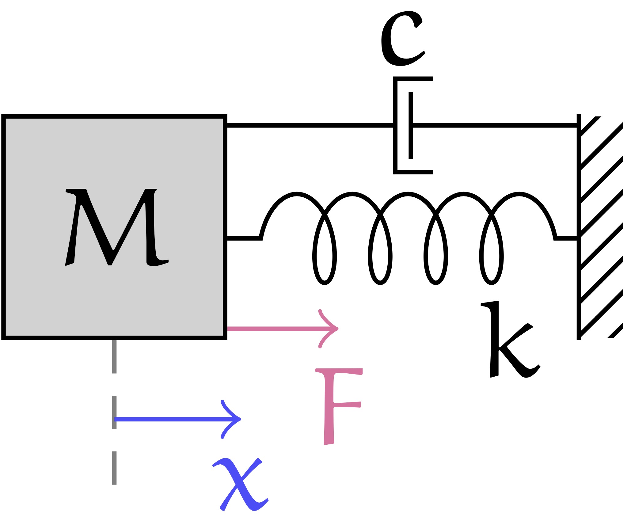
Mass-spring-damper Estimator

Mass-spring-damper example details

The system to be modeled is defined by the following equation:

\[M \ddot x = - k x - c \dot x + F\]

Build the neural model

Suppose we want to estimate the value of the future position of the mass, given the initial position and the external force. The MS-NN model is defined by a list of inputs and outputs, and by a list of relationships that link the inputs to the outputs. In nnodely, we can build an estimator in this form:

x = Input('x')
F = Input('F')
x_z_est = Output('x_z_est', Fir(x.tw(0.25)) + Fir(F.last()))

Input variables can be created using the Input function. In our system, we have two inputs: the position of the mass, x, and the external force exerted on the mass, F. The Output function is used to define a model’s output. The Output function has two inputs: the first is the name (string) of the output, and the second is the structure of the estimator.

Let us explain some of the functions used: The tw(...) function is used to extract a time window from a signal. In particular, we extract a time window \(T_w\) of 0.25 second. The last() function is used to get the last force sample applied to the mass, i.e., the force at the current time step. The Fir(...) function builds an FIR (finite impulse response) filter with one learnable parameter on our input variable. Hence, we are creating an estimator for the variable x at the next time step (i.e., the future position of the mass), by building an observer with the following mathematical structure:

\[x[1] = \sum_{k=0}^{N_x-1} x[-k]\cdot h_x[(N_x-1)-k] + F[0]\cdot h_F\]

where \(x[1]\) is the next position of the mass, \(F[0]\) is the last sample of the force, \(N_x\) is the number of samples in the time window of the input variable x, \(h_x\) is the vector of learnable parameters of the FIR filter on x, and \(h_f\) is the single learnable parameter of the FIR filter on F. For the input variable x, we are using a time window \(T_w = 0.25\) second, which means that we are using the last \(N_x\) samples of the variable x to estimate the next position of the mass. The value of \(N_x\) is equal to \(T_w/T_s\), where \(T_s\) is the sampling time used to sample the input variable x. In a particular case, our MS-NN formulation becomes equivalent to the discrete-time response (discretized with Forward-Euler) of the mass-spring-damper system. This happens when we choose the following values: \(N_x = 3\), \(h_x\) equal to the characteristic polynomial of the system, and \(h_f = T_s^2/m\), where \(T_s\) is the sampling time and \(m\) is the mass of the system. However, our formulation is more general and can better adapt to model mismatches and noise levels in the measured variables. This improved learning potential can be achieved by using a larger number of samples \(N_x\) in the time window of the input variable x. Let us now train our MS-NN observer using the available data. We perform:

mass_spring_damper = Modely()
mass_spring_damper.addModel('x_z_est', x_z_est)
mass_spring_damper.addMinimize('next-pos', Input('x_r').z(-1), x_z_est, 'mse')
mass_spring_damper.neuralizeModel(0.05)

The first line creates a nnodely object, while the second line adds one output to the model using the addModel function. To train our model, we use the function addMinimize to add a loss function to the list of losses. This function uses the following inputs: The first input is the name of the error (‘next-pos’ in this case). The second and third inputs are the variables whose difference we want to minimize. The fourth input is the loss function to be used, in this case the mean square error (‘mse’). In the function addMinimize, we apply the z(-1) method to the variable \(x\) to get the next position of the mass, i.e., the value of x at the next time step. The z(-1) function follows the Z-transform notation and is equivalent to a next() operator. The function z(...) can be used on an Input variable to obtain a time-shifted value. Hence, our training objective is to minimize the mean square error between \(x_z\), which represents the next position of the mass, and x_z_est, which represents the output of our estimator:

\[\frac{1}{n} \sum_{i=0}^{n} (x_{z_i} - x_{{z_est}_i})^2\]

where n represents the number of samples in the dataset.

Finally, the function neuralizeModel is used to create a discrete-time MS-NN model. The input parameter of this function is the sampling time \(T_s\), chosen based on the available data. In this example, \(T_s = 0.05\) seconds. The training dataset is then loaded. nnodely has access to all the files located in a source folder.

data_struct = ['time', ('x','x_r'), 'dx', 'F']
data_folder = os.path.join(os.path.dirname(os.path.realpath(__file__)),'dataset','data')
mass_spring_damper.loadData(name='mass_spring_dataset', source=data_folder, format=data_struct, delimiter=';')

Using the loaded dataset, we now train the neural model:

mass_spring_damper.trainModel()

After training the model, we test it using a new dataset. Let us create a simple example:

sample = {'F':[0.5], 'x':[0.25, 0.26, 0.27, 0.28, 0.29]}
results = mass_spring_damper(sample)
print(results)

Note that the input variable x is a list of 5 samples plus one sample, as the sampling time \(T_s\) is 0.05 seconds and the time window \(T_w\) of the input variable x is 0.25 second. For the input variable \(F\), we provide only one sample, since we use the last force value. The resulting output variable is structured as follows:

{'x_z_est':[0.3]}

where the value represents the output of our estimator, i.e., the next position of the mass.

Code

---

Reacher Estimator

Reacher details

Here is simple two-joint planar manipulator. The inputs are the joint angles \(\theta_1\) and \(\theta_2\), while the outputs are the end-effector coordinates \((x, y)\). The link lengths \(l_1\) and \(l_2\) are unknown and are estimated from data using nnodely as learnable parameters.

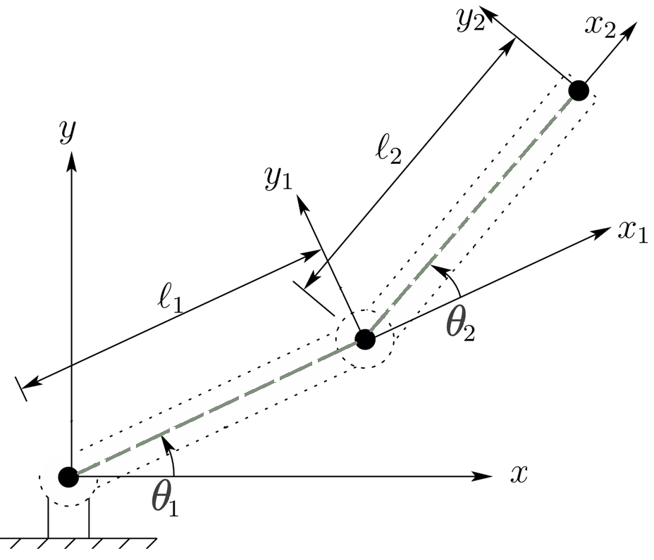
The kinematic model is given by:

\[x = l_1 \cos(\theta_1) + l_2 \cos(\theta_1 + \theta_2), \quad y = l_1 \sin(\theta_1) + l_2 \sin(\theta_1 + \theta_2).\]

Local Module Path Configuration and Package Import

First, we ensure Python can locate modules in the current working directory, enabling the import of nnodely components for use in the script.

import sys
import os
sys.path.append(os.getcwd())
from nnodely import *

Inputs from dataset & Parameters

Input variables are created using the Input class. The learnable parameters are given within the Parameter. The Output class defines the model output and takes two arguments: the name of the output and its structure.

# Inputs from dataset
theta1 = Input('theta1')
theta2 = Input('theta2')
x_tip  = Input('x_tip')
y_tip  = Input('y_tip')

l1 = Parameter('l1')  #parameters to be estimated
l2 = Parameter('l2')  #parameters to be estimated

x_out = Output('x_out', (l1 * Cos(theta1.last())) +
       (l2 * Cos(theta1.last() + theta2.last())))
y_out = Output('y_out', (l1 * Sin(theta1.last())) +
       (l2 * Sin(theta1.last() + theta2.last())))

Model composition

addModel adds the defined output to the model. addMinimize defines the loss function. This function uses the following inputs: The first input is the name of the error (x-error and y-error in this case). The second and third inputs are the variables whose difference we want to minimize. The fourth input is the loss function to be used, in this case the mean square error (mse). neuralizeModel builds the discrete-time MS-NN where its input parameter is the sampling time.

# Model composition
model = Modely(seed=0)
model.addModel('x_out', x_out)
model.addModel('y_out', y_out)
model.addMinimize('x-error', x_tip.last(), x_out, 'mse') # Objectives
model.addMinimize('y-error', y_tip.last(), y_out, 'mse') # Objectives
model.neuralizeModel(sample_time=0.02)

Data loading

nnodely requires two pieces of information: the data structure and the dataset location.

data_struct = ['step', 'T1','T2','theta1', 'theta2', 'x_tip', 'y_tip',
               'thetadot1', 'thetadot2', 'thetaddot1', 'thetaddot2'] # dataset creation

data_folder = os.path.join(os.getcwd(), 'dataset', 'data')

model.loadData(name='reacher_data', source=data_folder,
            format=data_struct, delimiter=';')  # Data loading

Training

Trains the model for 200 epochs (batch size 128, learning rate 0.01) using a 70/20/10 train-validation-test split.

# Training
train_params = {'num_of_epochs': 200, 'train_batch_size': 128, 'lr': 0.01}
model.trainModel(splits=[70, 20, 10], training_params=train_params)

Code

---

Applications

For additional examples, please refer to the nnodely Applications at the link below.

Applications Repository

---

Tutorials

For the tutorial please refer to the link below.

Tutorials